Plots
In this tutorial, we will explore how to plot the simulations generated by SWAMP-E.
All tutorials are available for download here.
[1]:
import os
import imageio
import numpy as np
from matplotlib import cm
import matplotlib.pyplot as plt
import SWAMPE
Let’s load the reference data. To make the path to the reference data work, it is easiest to download the notebooks by cloning the repository.
[2]:
# load  reference data
data_dir1 = os.path.abspath('../../../SWAMPE/reference_data/HJ_taurad_100/')+'\\'
timestamp1=710
eta1, delta1, Phi1, U1, V1 =SWAMPE.continuation.load_data(timestamp1,custompath=data_dir1)
data_dir2 = os.path.abspath('../../../SWAMPE/reference_data/HJ_taurad_0p1/')+'\\'
timestamp2=650
eta2, delta2, Phi2, U2, V2 =SWAMPE.continuation.load_data(timestamp2,custompath=data_dir2)

#generate the latitudes and longitude of matching resolution
M=42
N,I,J,dt,lambdas,mus,w=SWAMPE.initial_conditions.spectral_params(M)
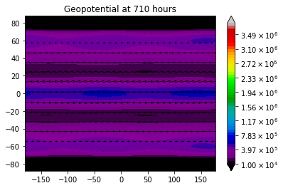
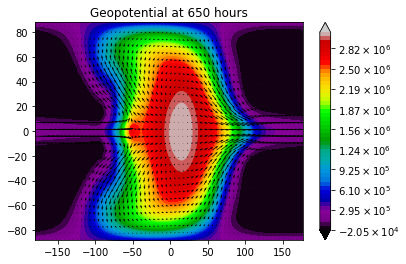
Plotting the geopotential plot with a wind vector field
[3]:
# plot the geopotential field with the overlayed wind field

fig1=SWAMPE.plotting.quiver_geopot_plot(U1,V1,Phi1,lambdas,mus,timestamp1)
fig2=SWAMPE.plotting.quiver_geopot_plot(U2,V2,Phi2,lambdas,mus,timestamp2)


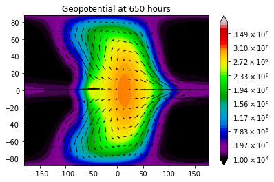
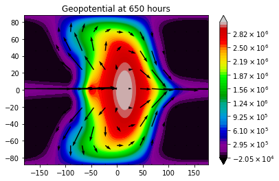
We can change the limits of the colorbar. This can be useful for comparing the outputs of multiple simulations.
[4]:
#change min/maxlevel
Phibar=4*10**6
fig1=SWAMPE.plotting.quiver_geopot_plot(U1,V1,Phi1,lambdas,mus,timestamp1,minlevel=10**4,maxlevel=3.8*10**6)
fig2=SWAMPE.plotting.quiver_geopot_plot(U2,V2,Phi2,lambdas,mus,timestamp2,minlevel=10**4,maxlevel=3.8*10**6)
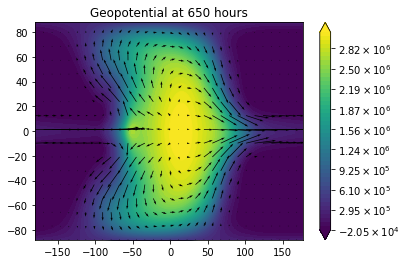
[5]:
#change colormap
colormap=cm.viridis
fig=SWAMPE.plotting.quiver_geopot_plot(U2,V2,Phi2,lambdas,mus,timestamp2,colormap=colormap)
We can also change the density of the wind vector field using sparseness.
[6]:
#change sparseness
sparsenessvec=[2,4,6,8]
for i in range(len(sparsenessvec)):
    fig=SWAMPE.plotting.quiver_geopot_plot(U2,V2,Phi2,lambdas,mus,timestamp2,sparseness=sparsenessvec[i])


We can also save the figure. By default, SWAMPE will create a “plots” directory in the current folder. You can also provide a custom path using the optional argument “custompath”.
[7]:
#save figure tutorial

fig=SWAMPE.plotting.quiver_geopot_plot(U2,V2,Phi2,lambdas,mus,timestamp2,savemyfig=True,filename='geopotfig.pdf')

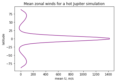
Plotting mean-zonal winds
Now let’s plot mean zonal winds:
[8]:
# plot mean zonal winds
fig1=SWAMPE.plotting.mean_zonal_wind_plot(U1,mus,timestamp1)
plt.show()
fig2=SWAMPE.plotting.mean_zonal_wind_plot(U2,mus,timestamp2,color='purple',customtitle='Mean zonal winds for a hot Jupiter simulation')

These plots can also be saved similarly to the quiver geopotential plots using “savemyfig”.
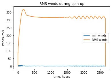
Plotting RMS winds during spinup
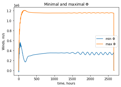
GCM simulations can take a while to run. SWAMPE can save spin-up data, specifically RMS wind data as well as the minimum and maximum geopotential.
[9]:
#load RMS winds
data_dir_spinup = os.path.abspath('../../../SWAMPE/reference_data/spinup_data/')+'\\'
spinup_winds=SWAMPE.continuation.read_pickle('spinup-winds',custompath=data_dir_spinup)
spinup_geopot=SWAMPE.continuation.read_pickle('spinup-geopot',custompath=data_dir_spinup)
[10]:
# plot RMS winds
SWAMPE.plotting.spinup_plot(spinup_winds,30)
#plot minimal and maximal geopotential
SWAMPE.plotting.spinup_plot(spinup_geopot,30,customlegend=['min $\Phi$','max $\Phi$'],customtitle='Minimal and maximal $\Phi$')
[10]:
[<matplotlib.lines.Line2D at 0x2fb13effbe0>]
Creating gifs
While many simulations converge to a constant steady-state, in many settings, oscillations are present. In these circumstances, it can be helpful to combine several snapshots into a gif.
[12]:
## make a geopotential gif
num_snapshots=11
timestamps=np.zeros(num_snapshots)

Phidata=np.zeros((num_snapshots,J,I))
Udata=np.zeros((num_snapshots,J,I))
Vdata=np.zeros((num_snapshots,J,I))

#load data
data_dir3 = os.path.abspath('../../../SWAMPE/reference_data/SN_for_gif/')+'\\'


for i in range(num_snapshots):
    timestamp=int(2500+10*i)
    timestamps[i]=timestamp
    eta, delta, Phi, U, V =SWAMPE.continuation.load_data(timestamp,custompath=data_dir3)
    Phidata[i,:,:]=Phi
    Udata[i,:,:]=U
    Vdata[i,:,:]=V
To generate a gif, we run the following code:
SWAMPE.plotting.write_quiver_gif(lambdas,mus,Phidata,Udata,Vdata,timestamps,'testgif.gif',sparseness=4,frms=5)
The resulting gif should look like this: