SWAMPE Quick Start

In this tutorial, we will explore how to use SWAMP-E to simulate planetary atmospheres.

All tutorials are available for download here.

import numpy
import SWAMPE

Running SWAMPE

Planetary Parameters

First, let’s specify some key physical inputs:

# planetary radius a in meters

a=8.2*10**(7)

# planetary rotation rate omega in radians/s

omega=3.2*10**(-5)

# the reference geopotential height, m^2/s^2, typically based on scale height

Phibar=4*(10**6)

Simulation Parameters

Now let’s specify the timestep and the number of timesteps. For stability, a reasonable timestep will range from 30 to 180 seconds, with strongly forced planets needing a shorter timestep.

#timestep length in seconds
dt=30
#number of timesteps for the simulation
tmax=10

We will also specify the spectral resolution M. This resolution determines the size of the resulting lat-lon grid.

M=42

Forcing parameters

Let’s specify forcing parameters. The forcing strength is controlled via DPhieq, which is the day/night amplitude of the local radiative equilibrium geopotential. The default forcing scheme in SWAMPE is based on Perez-Becker and Showman (2013). The current default forcing scheme supports synchronous rotators with time-constant stellar irradiation. If you’d like to simulate other forcing patterns, download SWAMPE from the repository and change SWAMPE.forcing.Phieqfun (prescribing local radiative equilibroum) and/or SWAMPE.forcing.Qfun (the Newtonian relaxation to local radiative equilibrium).

We also specify two timescales: a radiative timescale of one day and a drag timescale of ten days.

DPhieq=Phibar

taurad=3600*24
taudrag=10*3600*24

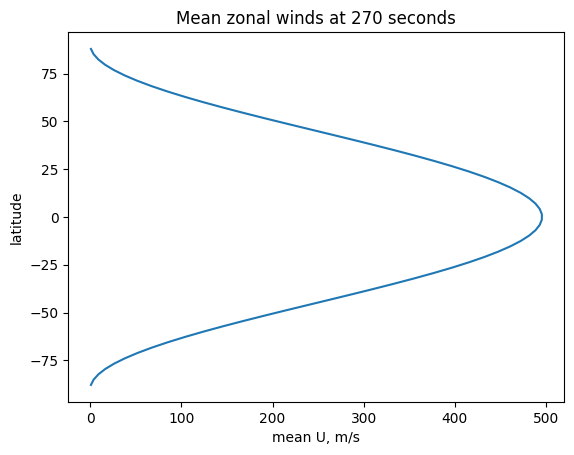
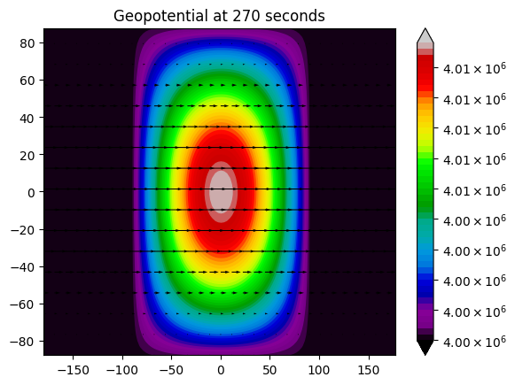
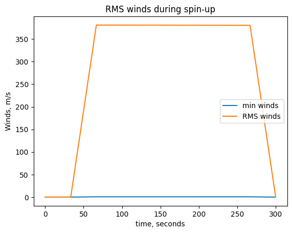
Now, we can use SWAMP-E to run the simulation. We can specify whether we want to see plots as the simulation is conducted and control the frequency of output using plotflag and plotfreq.

plotflag=True
plotfreq=9 #output plots every 9 time steps

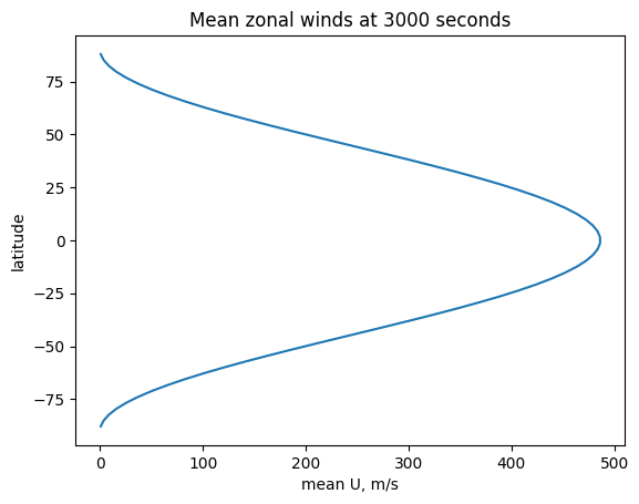
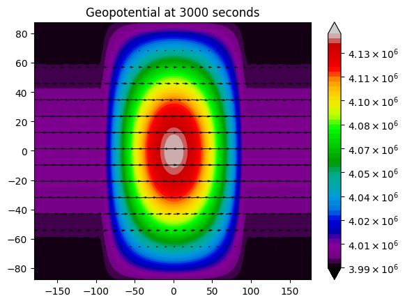
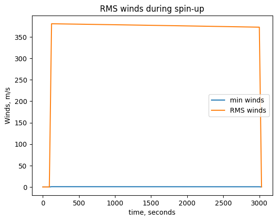
SWAMPE.run_model(M,dt,tmax,Phibar, omega, a,  taurad=taurad, taudrag=taudrag, DPhieq=DPhieq, plotflag=plotflag, plotfreq=plotfreq,saveflag=False,verbose=False,timeunits='seconds')

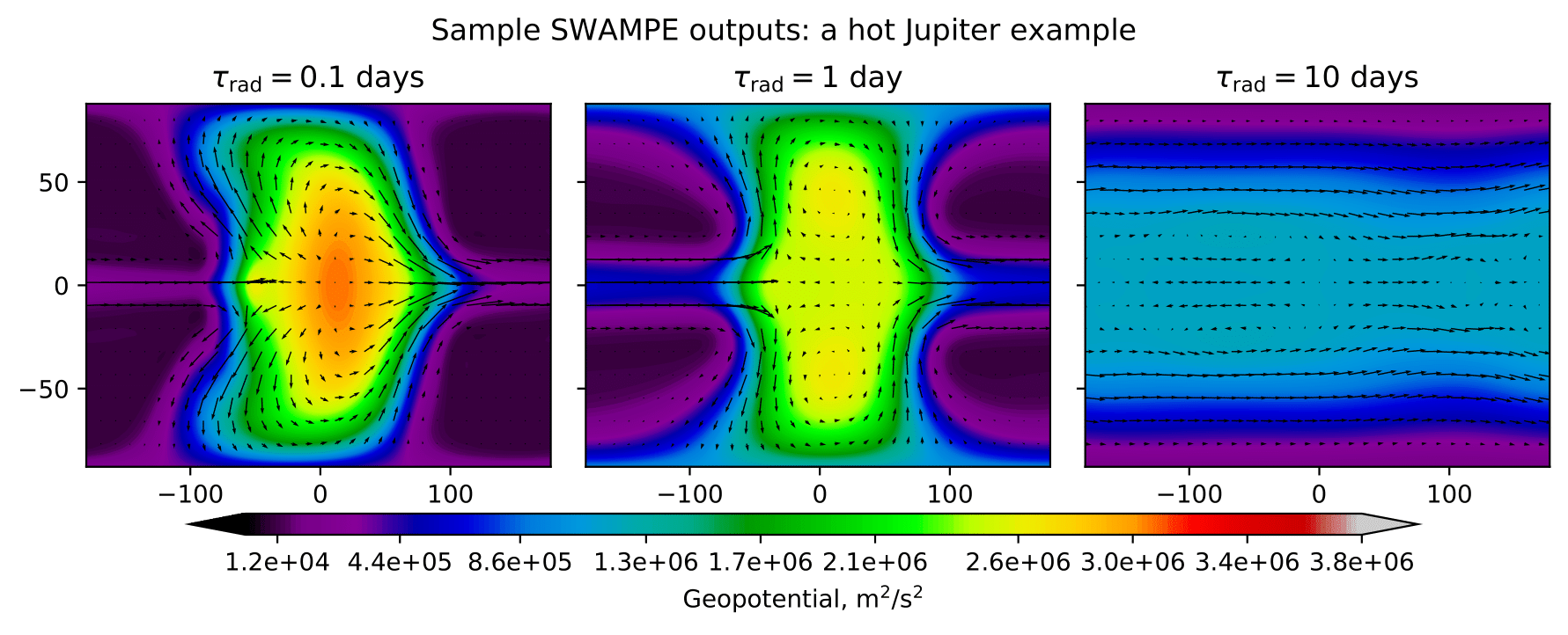
Note that a 2D model like SWAMP-E will need a few hundred time steps to spin up, so with a real-world example, we recommend running the model using a script rather than a Jupyter notebook. Here are sample outputs for the same planetary parameters, but without drag (equivalent to \(\tau_{\rm drag}=\infty\)) and with \(\tau_{\rm rad}\) equal to 0.1, 1, and 10 Earth days. The scripts and the reference data are provided here.

Saving and loading SWAMPE data

Saving the data

Since the simulations can take a few hundred timeteps to spin up, it is helpful to save the data to be loaded later. We can specify whether to save the data using saveflag. We can also specify savefrequency. The data will be stored in the pickle format with the name ‘variable-timestamp’, where timestamp can be specified in seconds, minutes, or hours.

The saved data files will look like this:

Phi-10
eta-10
delta-10
U-10
V-10

This will save the data every 120 time steps in the folder C:/your/Path/here/

SWAMPE.run_model(..., saveflag=True, savefreq=120, custompath='C:/your/Path/here/',timeunits='minutes')

For a timestep of 30 seconds, the first output will look like this, with the timestamp of sixty minutes:

Phi-60
eta-60
delta-60
U-60
V-60

If no custom path is provided, SWAMPE will create a local ‘data/’ directory and store the data there.

Continuation

We can also start the simulation from any suitable initial condition. Let’s save some data and restart the simulation from the saved data.

#saving the data every 5 timesteps
SWAMPE.run_model(M,dt,tmax,Phibar, omega, a,  taurad=taurad, taudrag=-1, DPhieq=Phibar, plotflag=False, plotfreq=plotfreq,saveflag=True,savefreq=5,verbose=False,timeunits='seconds')
#note taudrag=-1 corresponds to taudrag=infinity, or no drag

Now we can load the saved data. Let’s say we want to load the data from 150 seconds.

timestamp='150'
eta, delta, Phi, U, V =SWAMPE.continuation.load_data(str(timestamp))

N,I,J,otherdt,lambdas,mus,w=SWAMPE.initial_conditions.spectral_params(M)
fig=SWAMPE.plotting.quiver_geopot_plot(U,V,Phi+4*10**6,lambdas,mus,timestamp,sparseness=4,minlevel=None,maxlevel=None,units='seconds')

SWAMPE.run_model(M,30,101,Phibar, omega, a,  taurad=taurad, taudrag=-1, DPhieq=Phibar, plotflag=True, plotfreq=100,saveflag=False,verbose=True,timeunits='seconds',contflag=True,contTime=150)

t=10, 9.900990099009901% complete
t=20, 19.801980198019802% complete
t=30, 29.702970297029704% complete
t=40, 39.603960396039604% complete
t=50, 49.504950495049506% complete
t=60, 59.40594059405941% complete
t=70, 69.3069306930693% complete
t=80, 79.20792079207921% complete
t=90, 89.10891089108911% complete
t=100, 99.00990099009901% complete

GCM run completed!